\(
\def\pause{}
\def\,{\kern.2em}
\def\implies{\Longrightarrow}
\newcommand{\alert}[1]{\color{red}{#1}}
\def\ds{\displaystyle}
\let\epsilon\varepsilon
\let\subseteq\subseteqq
\let\supseteq\supseteqq
\let\setminus\smallsetminus
\let\le\leqq
\let\leq\leqq
\let\ge\geqq
\let\geq\geqq
\newcommand{\NN}{\mathbb N}
\newcommand{\RR}{\mathbb R}
\renewcommand{\limsup}{\mathop{\overline{\mathrm{lim}}}}
\renewcommand{\liminf}{\mathop{\underline{\mathrm{lim}}}}
\newcommand{\redlimsup}{\mathop{\color{red}{\overline{\mathrm{lim}}}}}
\newcommand{\redliminf}{\mathop{\color{red}{\underline{\mathrm{lim}}}}}
\newcommand{\konv}[1][]{\mathbin{\mathop{\longrightarrow}\limits_{#1}}}
\newcommand{\bigset}[2]{\left\{{#1}\left|\strut
\vphantom{#1}\vphantom{#2}\right.\, {#2}\right\}}
\newcommand{\set}[2]{\left\{\smash{#1}\left|%
\vphantom{\smash{#1}}\vphantom{\smash{#2}}\right.\,\smash{#2}\right\}}
\newcommand{\E}{\mathrm{e}}
\newcommand{\I}{\mathrm{i}}
\newcommand{\diff}{\mathop{\mathrm{\kern0pt d}}}
\newcommand{\diffAt}[3]{\frac{\diff}{\diff{#2}}\,\left.{\vphantom{\frac00}#1}\,\right|_{#2=#3}}
\newcommand{\partAt}[3]{\frac{\partial}{\partial{#2}}\,\left.{\vphantom{\frac00}#1}\,\right|_{#2=#3}}
\newcommand{\diffgleich}{\mathbin{\,\mathop{=}\limits^{\,\prime}}\,}
\newcommand{\grad}{\mathop{\mathrm{grad}}}
\newcommand{\Jac}[2]{\mathrm{J}{#1}\left(#2\right)}
\newcommand{\Hesse}[2]{\mathrm{H}{#1}\left(#2\right)}
\newcommand{\Hesso}[1]{\mathrm{H}{#1}}
\newcommand{\Bar}[1]{\overline{#1}}
\newcommand{\transp}{^{^{\scriptstyle\intercal}}}
\newcommand{\inn}[1]{{#1}^\circ}
\newcommand{\Cf}[2]{\mathcal C^{#1}(#2)}
\newcommand{\skalp}{\mathbin{\scriptstyle\bullet}}
\newcommand{\IA}{{\sf\color{DarkGreen}{(IA)}}}
\newcommand{\IH}{{\sf\color{DarkGreen}{(IH)}}}
\newcommand{\IS}{{\sf\color{DarkGreen}{(IS)}}}
\)
Für alle \(x\in\RR\) mit \(x \gt -1\)
und alle \(n\in\NN_0\) gilt:
\(
1+n\,x \le (1+x)^n
\).
0.5.2 Schwarzsche Ungleichung
Für beliebige \(a_j,b_j\in\RR\) gilt
\(
\biggl(\sum\limits_{j=1}^n a_j\,b_j\biggr)^2 \leqq
\biggl(\sum\limits_{j=1}^n a_j^2\biggr)
\biggl(\sum\limits_{j=1}^n b_j^2\biggr)
\).
0.5.3 Arithmetisches und geometrisches Mittel
Für beliebige \(a_1,\ldots,a_n\in\RR^+_0\) gilt
\(
\ds\frac{a_1+\cdots+a_n}n \ge \sqrt[n]{\strut a_1\cdots a_n} \,.
\)
Man nennt \(\ds\frac{a_1+\cdots+a_n}n\) das arithmetische
und \(\sqrt[n]{a_1\cdots a_n}\) das geometrische Mittel.
Mit Hilfe des Höhensatzes kann man die Ungleichung veranschaulichen:
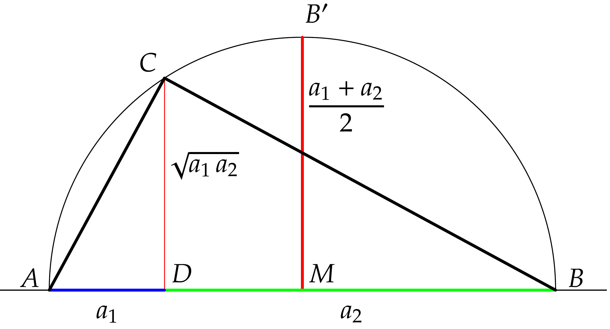
Die Strecke \(\Bar{A\,D}\) habe die Länge \(a_1\), die Strecke \(\Bar{D\,B}\) die
Länge \(a_2\). Wir errichten die Lote im Mittelpunkt \(M\) von \(\Bar{A\,B}\) und
in \(D\), diese treffen den Thaleshalbkreis über \(\Bar{A\,B}\) in \(B'\)
bzw. \(C\).
Nach dem Höhensatz ist das Quadrat der
Länge von \(\Bar{C\,D}\) gleich \(a_1\,a_2\).